Valuation Bond Pricing using Vasicek Model

Vasicek model

The Vasicek model is a popular short-rate model used in financial mathematics to describe the evolution of interest rates. It is defined by the following stochastic differential equation (SDE): \[dr_t = a(b - r_t)dt + \sigma dW_t \] where: - $r_t$ is the short-term interest rate at time $t$, - $a$ is the speed of mean reversion, - $b$ is the long-term mean level, - $\sigma$ is the volatility of the interest rate, - $W_t$ is a standard Wiener process (Brownian motion).

Import Libraries

Code

import numpy as np
import matplotlib.pyplot as plt
import pandas as pd
import seaborn as sns
import datetime
from scipy.stats import linregress
from scipy.stats import norm
import statsmodels.api as sm

1. Load Interest Rate Data

Code

import pandas_datareader.data as web

start_date = datetime.datetime(2020, 1, 1)
end_date = datetime.datetime(2025, 12, 31)

df = web.DataReader('DTB3', 'fred', start_date, end_date)

Code

# data = web.DataReader('DGS1', 'fred', start_date, end_date)
# data = data.dropna()
# data.index = pd.to_datetime(data.index)
# data.head()

Code

import yfinance as yf
symbol = "^TNX"
start_date = "2012-01-01"
end_date = "2024-01-31"

data = yf.download(symbol, start=start_date, end=end_date)
data = data['Close'].dropna()

rate = data.values

plt.figure(figsize=(12,4))
plt.plot(data, label='10-Year Treasury Yield')
plt.title('10-Year Treasury Yield Over Time')
plt.xlabel('Date')
plt.ylabel('Yield')
plt.legend()
plt.show()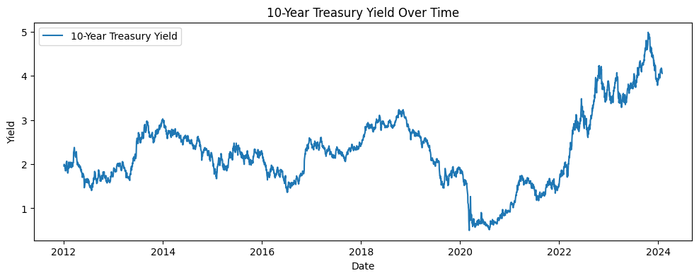

Code

df = data.copy()

Code

df.head()

Ticker	^TNX
Date
2012-01-03	1.960
2012-01-04	1.995
2012-01-05	1.993
2012-01-06	1.961
2012-01-09	1.960

Code

df.info()

<class 'pandas.core.frame.DataFrame'>
DatetimeIndex: 3037 entries, 2012-01-03 to 2024-01-30
Data columns (total 1 columns):
 #   Column  Non-Null Count  Dtype  
---  ------  --------------  -----  
 0   ^TNX    3037 non-null   float64
dtypes: float64(1)
memory usage: 47.5 KB

Code

df = df.dropna()
df.index = pd.to_datetime(df.index)
df.head()

Ticker	^TNX
Date
2012-01-03	1.960
2012-01-04	1.995
2012-01-05	1.993
2012-01-06	1.961
2012-01-09	1.960

Code

plt.figure(figsize=(12, 6))
sns.lineplot(data=df, x=df.index, y='^TNX')
plt.title('10-Year Treasury Yield')
plt.xlabel('Date')
plt.ylabel('Rate (%)')
plt.grid(True)
plt.show()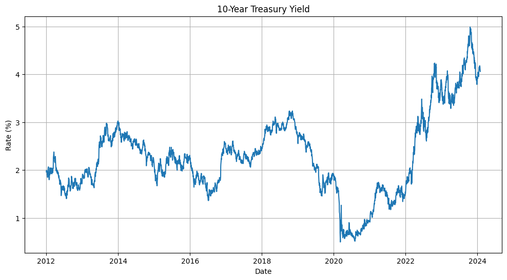

2. Estimate Vasicek Model Parameters

OLP Calibrtion Method:

We can calibrate the Vasicek model using standard Linear Regression (Ordinary Least Squares - OLS).

The dicrete Euler equation for the Vasicek model is given by: \[r_{t+1}-r_t = a(b-r_t)\Delta t + \sigma \sqrt{\Delta t} \epsilon_t \]

We can rewrite it to look like a linear regression equation: $(Y=+ X + ) $

\[\underbrace{r_{t+1}}_{Y} = \underbrace{ab\Delta t}_{\alpha} + \underbrace{(1 - a\Delta t)}_{\beta} \underbrace{r_t}_{X} + \underbrace{\sigma \sqrt{\Delta t} \epsilon_t}_{\text{noise}} \]

Where $\epsilon_t$ is a standard normal random variable.

By running a regression of the change in rate $(Y)$ against the current rate $(X)$, we find estimates for $\alpha$ and $\beta$.

Speed of Reversion $(a)$ : $a = \dfrac{1 - \beta}{\Delta t}$
Long-term Mean Level $(b)$ : $b = \dfrac{\alpha}{a \Delta t}$
Volatility $(\sigma)$ : The standard deviation of the residuals from the regression gives us $\sigma \sqrt{\Delta t}$, so we can compute $\sigma$ as: $

Code

def calibrate_vasicek(rates, dt=1/252):
    """
    Calibrates a, b, sigma using OLS on discretized SDE:
    r_{i+1} = a*b*dt + (1 - a*dt)*r_i + sigma*sqrt(dt)*eps
    """
    y = rates.values[1:]
    x = rates.values[:-1]
    X = sm.add_constant(x)
    
    model = sm.OLS(y, X).fit()
    alpha, beta = model.params
    residuals_std = np.std(model.resid)
    
    # Extract parameters from regression coefficients
    a = (1 - beta) / dt
    b = alpha / (a * dt)
    sigma = residuals_std / np.sqrt(dt)
    
    return a, b, sigma

Code

rates = df['^TNX'] / 100
a, b, sigma = calibrate_vasicek(rates,dt=1/252)

print(f"Calibrated Vasicek parameters:")
print(f"a (speed of reversion): {a}")
print(f"b (long-term mean): {b}")
print(f"sigma (volatility): {sigma}")

Calibrated Vasicek parameters:
a (speed of reversion): 0.2911154424136324
b (long-term mean): 0.028783115580092614
sigma (volatility): 0.00816174293304405

Code

# Optional: Visualize the fit
plt.figure(figsize=(12, 6))
plt.plot(df.index, df['^TNX']/100, label='Historical Rates')
plt.axhline(y=b, color='r', linestyle='--', label=f'Calibrated Mean (b={b:.1%})')
plt.title("Historical Short Rates vs. Calibrated Long-Term Mean")
plt.legend()
plt.grid()
plt.show()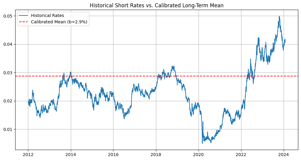

3. Simulate Interest Rate Paths

To simulate the short rate $r_t$ using the Vasicek model, we can use the following discretized version of the SDE: \[r_{t+\Delta t} = r_t + a(b - r_t)\Delta t + \sigma \sqrt{\Delta t} Z_t\]

where $Z_t$ is a standard normal random variable.

Code

def simulate_vasicek_paths(r0, a, b, sigma, T, dt, n_paths):
    n_steps = int(T / dt)
    rates = np.zeros((n_steps + 1, n_paths))
    rates[0] = r0
    
    for t in range(1, n_steps + 1):
        # dz ~ N(0, sqrt(dt))
        dz = np.random.normal(0, np.sqrt(dt), n_paths)
        # dr = a(b - r)dt + sigma * dW
        rates[t] = rates[t-1] + a * (b - rates[t-1]) * dt + sigma * dz
        
    return rates

Code

# Simulation parameters
r0 = rates[-1]
T = 1.0  # 1 year
dt = 1/252  # daily steps
n_paths = 1000  # number of simulated paths

rates_sim = simulate_vasicek_paths(r0, a, b, sigma, T, dt, n_paths)
time_grid = np.linspace(0, T, int(T/dt) + 1)

mean_rates = np.mean(rates_sim, axis=1)
plt.figure(figsize=(10, 6))
plt.plot(time_grid, rates_sim[:, :50], lw=1) 
plt.plot(time_grid, mean_rates, lw=2, color='blue')
plt.title('Simulated Interest Rate Paths (Vasicek Model)')
plt.xlabel('Time (years)')
plt.ylabel('Interest Rate (%)')
plt.axhline(y=b, color='r', linestyle='--', label='Long-term Mean (b)')
plt.text(0.1, b - 0.003, f'b = {b:.4f}', color='r')
plt.legend()
plt.grid(True)
plt.show()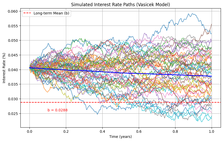

4. Price Zero-Coupon Bonds

The price of a zero-coupon bond in the Vasicek model can be calculated using the following formula: \[P(t,T) = A(t,T) e^{-B(t,T) r_t}\] where: - $P(t,T)$ is the price of the bond at time $t$ maturing at time $T$, - $A(t,T)$ and $B(t,T)$ are functions defined as:

\[B(t,T) = \dfrac{1 - e^{-a(T-t)}}{a}\]

\[A(t,T) = \exp\left( \left( b - \dfrac{\sigma^2}{2a^2} \right) \left( B(t,T) - (T-t) \right) - \dfrac{\sigma^2 B(t,T)^2}{4a} \right)\]

Code

def analytical_bond_price(r, a, b, sigma, T):
    B = (1 - np.exp(-a * T)) / a
    A = np.exp((B - T) * (a**2 * b - 0.5 * sigma**2) / a**2 - (sigma**2 * B**2) / (4 * a))
    P = A * np.exp(-B * r)
    return P

T_bond = 1.0  # 1 year bond
bond_prices = analytical_bond_price(r0, a, b, sigma, T_bond)
print(f"Analytical price of a zero-coupon bond maturing in {T_bond} year(s): {bond_prices:.4f}")

Analytical price of a zero-coupon bond maturing in 1.0 year(s): 0.9617

5. Monte Carlo Simulation for Bond Pricing

To estimate the price of a Zero-Coupon Bond (ZCB) using Monte Carlo simulation, we can follow these steps:

The price of a bond is the risk-neutral expectation of the discounted payoff:

\[P(0,T) = E^Q\left[e^{-\int_0^T r_t dt}\right]\]

In our simulation, the integral becomes a sum, and the expectation is approximated by the average over many simulated paths.

\[P_{MC} \approx \dfrac{1}{N} \sum_{i=1}^{N}\left( \exp \left(-\sum_{j=0}^{M-1} r_{t_j}^{(i)} \Delta t \right)\right)\]

Code

def price_bond_mc(rates, dt):
    # Stochastic Discount Factor: exp(-integral of r_t dt)
    integral_r = np.sum(rates[:-1, :], axis=0) * dt
    payoffs = np.exp(-integral_r)
    return np.mean(payoffs)

# Price a 1-year bond
T_target = 1.0
steps_target = int(T_target / dt)
mc_price = price_bond_mc(rates_sim[:, :], dt)
analyt_price = analytical_bond_price(r0, a, b, sigma, T_target)

print(f"--- Comparison  ---")
print(f"Analytical Price (1Y): {analyt_price:.5f}")
print(f"Monte Carlo Price (1Y): {mc_price:.5f}")
print(f"Error: {abs(mc_price - analyt_price):.5f}")

--- Comparison  ---
Analytical Price (1Y): 0.96173
Monte Carlo Price (1Y): 0.96175
Error: 0.00001

5.2 Compare

Code

# Parameters
T_max = 10
dt = 1/252


maturities = np.arange(1,T_max+1)
analytical_prices = [analytical_bond_price(r0, a, b, sigma, T) for T in maturities]

# Monte Carlo
n_paths = 1000
mc_prices = []
for T in maturities:
    full_paths = simulate_vasicek_paths(r0, a, b, sigma, T, dt, n_paths)
    integral_r = np.sum(full_paths, axis=0)*dt
    mc_prices.append(np.mean(np.exp(-integral_r)))

plt.figure(figsize=(10, 5))
plt.plot(maturities, analytical_prices, 'o-', label='Analytical Price', markersize=8)
plt.plot(maturities, mc_prices, 'x--', label=f'Monte Carlo Price (N={n_paths})', markersize=8)
plt.title("Task 3: Analytical vs. Monte Carlo Bond Prices")
plt.xlabel("Maturity (Years)")
plt.ylabel("Price")
plt.legend()
plt.grid(True)
plt.show()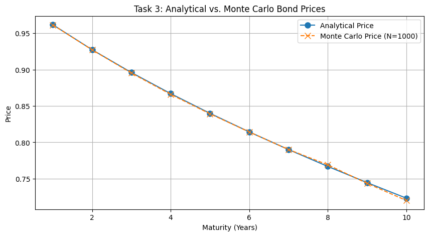

Code

absolute_errors = [abs(ap - mp) for ap, mp in zip(analytical_prices, mc_prices)]

comparison_df = pd.DataFrame({
    'Maturity (Years)': maturities,
    'Analytical Price': analytical_prices,
    f'Monte Carlo Price (N={n_paths})': mc_prices,
    'Absolute Error': absolute_errors
})

comparison_df

	Maturity (Years)	Analytical Price	Monte Carlo Price (N=1000)	Absolute Error
0	1	0.961734	0.961529	0.000205
1	2	0.927366	0.927190	0.000176
2	3	0.896006	0.895275	0.000731
3	4	0.867007	0.865980	0.001027
4	5	0.839894	0.839199	0.000695
5	6	0.814320	0.814280	0.000040
6	7	0.790027	0.790127	0.000099
7	8	0.766825	0.769030	0.002205
8	9	0.744570	0.743563	0.001008
9	10	0.723155	0.719999	0.003156

6. Yield Curve Analysis

Using the analytical bond pricing formula, generate the yield curve for different maturities $ T $ by calculating the yield $ y(0,T) $: \[ y(0,T) = -\frac{1}{T} \ln(P(0,T)) \]

Analyze how changes in parameters $ a $, $ b $, and $ $ affect the shape of the yield curve.

Code

maturities = np.linspace(0.1, 10, 100)

def get_yields(a, b, sigma):
    prices = [analytical_bond_price(r0, a, b, sigma, T) for T in maturities]
    return -np.log(prices) / maturities

Code

plt.figure(figsize=(12, 8))
plt.plot(maturities, get_yields(a, b, sigma), label='Base Case', lw=2)
plt.title("Base Yield Curve")
plt.xlabel("Maturity")
plt.ylabel("Yield")
plt.tight_layout()
plt.show()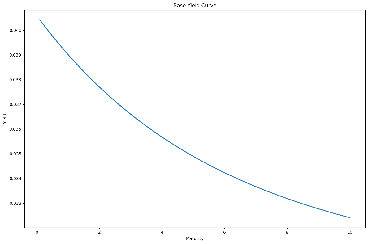

Code

plt.figure(figsize=(12, 5))
plt.subplot(1, 2, 1)

a_imp = [a/2, a, a*2]
for a_val in a_imp:
    yields = get_yields(a_val, b, sigma)
    plt.plot(maturities, yields, label=f'a={a_val:.4f}')
plt.title("Impact of Mean Reversion Speed (a)")
plt.xlabel("Maturity (Years)")
plt.ylabel("Yield")
plt.legend()
plt.grid(True)

# Scenario B: Effect of 'sigma' (Volatility)
sigma_imp = [sigma/2, sigma, sigma*2]
plt.subplot(1, 2, 2)
for sig_val in sigma_imp:
    yields = get_yields(a, b, sig_val)
    plt.plot(maturities, yields, label=f'sigma={sig_val:.4f}')
plt.title("Impact of Volatility (sigma)")
plt.xlabel("Maturity (Years)")
plt.ylabel("Yield")
plt.legend()
plt.grid(True)

plt.tight_layout()
plt.show()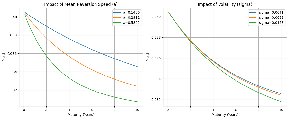

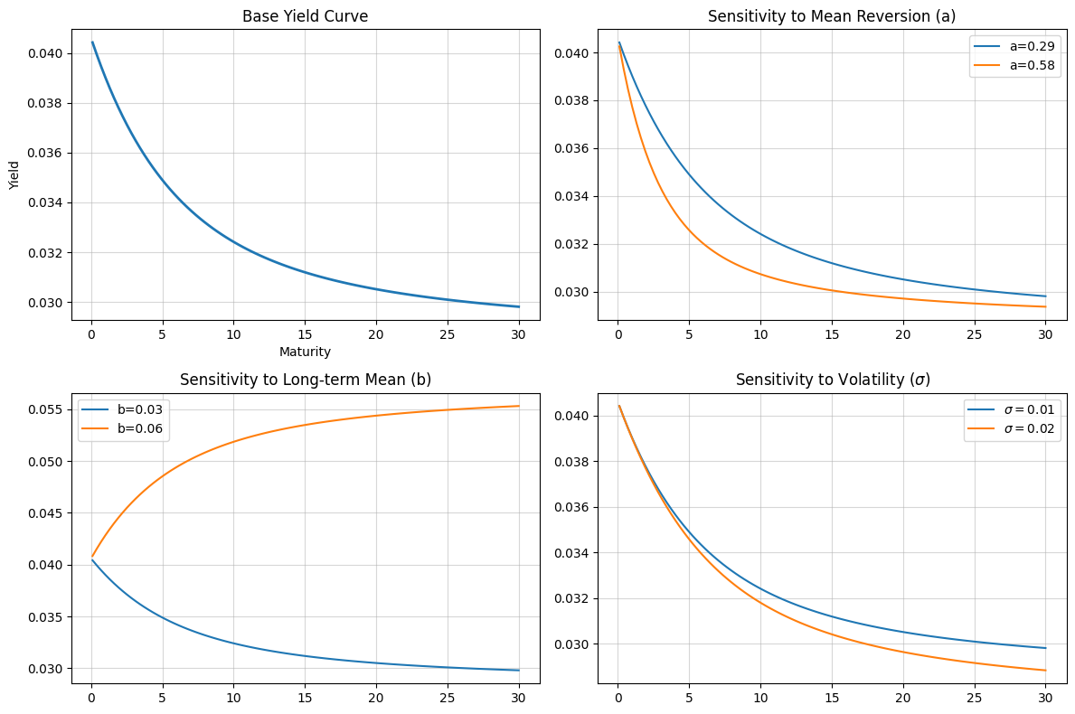
Code

# Task 4: Yield Curve and Sensitivity
m_yields = np.linspace(0.1, 30, 100)
def get_yields(a, b, sigma):
    prices = [analytical_bond_price(r0, a, b, sigma, T) for T in m_yields]
    return -np.log(prices) / m_yields

plt.figure(figsize=(12, 8))
plt.subplot(2, 2, 1)
plt.plot(m_yields, get_yields(a, b, sigma), label='Base Case', lw=2)
plt.title("Base Yield Curve")
plt.xlabel("Maturity")
plt.ylabel("Yield")
plt.grid(alpha=0.5)

plt.subplot(2, 2, 2)
plt.plot(m_yields, get_yields(a, b, sigma), label=f'a={a:.2f}')
plt.plot(m_yields, get_yields(2*a, b, sigma), label=f'a={2*a:.2f}')
plt.title("Sensitivity to Mean Reversion (a)")
plt.legend()
plt.grid(alpha=0.5)

plt.subplot(2, 2, 3)
plt.plot(m_yields, get_yields(a, b, sigma), label=f'b={b:.2f}')
plt.plot(m_yields, get_yields(a, 2*b, sigma), label=f'b={2*b:.2f}')
plt.title("Sensitivity to Long-term Mean (b)")
plt.legend()
plt.grid(alpha=0.5)

plt.subplot(2, 2, 4)
plt.plot(m_yields, get_yields(a, b, sigma), label=f'$\sigma={sigma:.2f}$')
plt.plot(m_yields, get_yields(a, b, 2*sigma), label=f'$\sigma={2*sigma:.2f}$')
plt.title("Sensitivity to Volatility ($\sigma$)")
plt.legend()
plt.grid(alpha=0.5)
plt.tight_layout()
plt.show()