The Vasicek Model

Mathematical Formulation

The Vasicek model (1977) assumes the process evolves as an Ornstein-Uhlenbeck process with constant coefficients:

\[ dr_t = \kappa(\theta - r_t)dt+\sigma dW_t \]

Parameters

• \(\kappa\): Speed of mean reversion.
• \(\theta\): Long-term mean level of the interest rate.
• \(\sigma\): Instantaneous volatility.

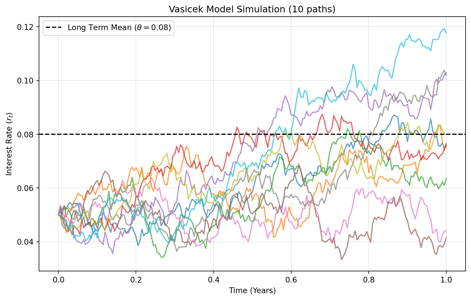
Python Simulation

We simulate the path using the Euler-Maruyama discretization method.

import numpy as np 
import matplotlib.pyplot as plt 

# 1. Set Parameters
r0 = 0.05
theta = 0.08
kappa = 0.5
sigma = 0.03
T =1.0
dt = 0.005
N = int(T / dt)
num_paths = 10

# 2. Simulation Loop
t = np.linspace(0, T, N+1)
rates = np.zeros((N+1, num_paths))
rates[0, :] = r0

np.random.seed(42)

for i in range(1, N+1):
    dw = np.random.normal(size=num_paths)
    dr = kappa * (theta - rates[i-1, :]) * dt + sigma * np.sqrt(dt) * dw
    rates[i, :] = rates[i-1, :] + dr

# 3. Visualization
plt.figure(figsize=(10, 6))
plt.plot(t, rates, lw=1.5, alpha=0.7)
plt.axhline(theta, color='black', linestyle='--', label=f'Long Term Mean ($\\theta={theta}$)')
plt.title(f'Vasicek Model Simulation ({num_paths} paths)')
plt.xlabel('Time (Years)')
plt.ylabel('Interest Rate ($r_t$)')
plt.legend()
plt.grid(True, alpha=0.3)
plt.show()